
Deep Reinforcement Learning for CartPole
In this session we will discuss about the Deep Reinforcement Learning (DRL). This is a machine learning/deep learning techniques where the system learns from its action like the way human learn by experience. In reinforcement learning, the agent is rewarded or penalized according to its action. If the action paves the way to target outcome, the agent will be rewarded. So the agent learns through trial and error in a dynamic environments.
In the below figure summarize the different between the Q-learning and the Deep Q-learning. In the RL, the agent use Q function to decide what action to take in the next step. In the Deep Q learning, we simply replace the Q table with a Deep Neural Networks (DNN).

In this lab we will solve CartPole problem (cotinuous input, discrete actions) using DQN. CartPole is nothing but an inverted pendulum with the center of mass above from the pivot point. A typical diagram of a CartPole can be seen below;

So naturally this physical system is unbalanced/unstable. It will tend to turn around with respect to the pivot point. The goal here is to balance CartPole by applying necessary forces to the pivot (to the right/left). If the pole is balanced, +1 is given in every time step. If the pole goes away from a certain angle with respect to the vertical, the game ends. We can see a real world demonstration here.
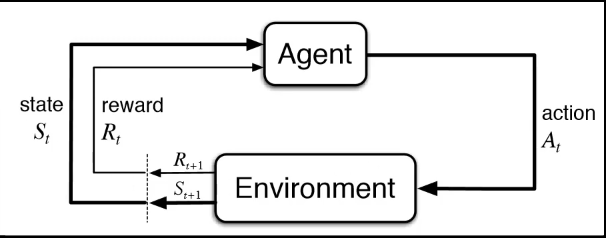
The following figure shows how the agent interact with the environment, this is known as Markov chain. It shows an agent takes an action at a time t on the environment. Based on the action, the agent gets a reward as well as move to a new state at time t+1. So in each iteration, the agent takes the current state, get the best action and execute in in the environment.
First let us import the necessary libraries and declare the environment.

Let us see how to define the agent neural networks (QNetwork). This can be used to obtained Q value for a specific action.


Now let us define the Doer class!! The Doer class is responsible for the action of the agent. The following class is the Doer implementation.
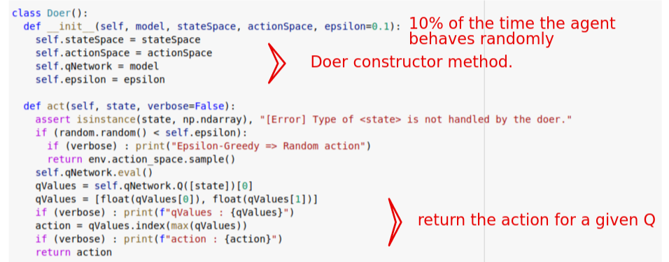
Now let us test this Doer class. The following is the output of the Doer class;

Transition Class
The following class is used to get the state & action from one time frame to another. From the current state(St), current action(At) to the next state (Stp) & action (Atp). Also it checks whether all these At,St,Atp,Stp are None. To sum up, it essentially maps (state, action) pairs to their (next_state, reward) result (ref 4).
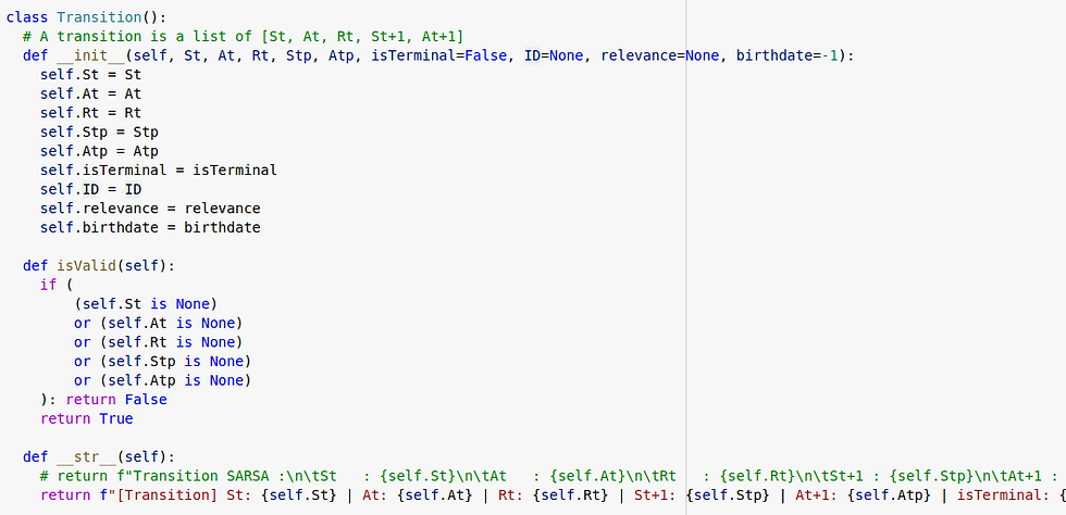
The following is the out put of the class Transition.

Experience Replay and Replay Memory
During the training of the DQN, we use a technique called "experience replay". The idea behind this is that we store the agent's experience at each time interval in "replay memory". If we represent the agent's experience by e_t at a time step t. Then it can be defined as
e_t = (s_t, a_t, r_t+1, s_t+1)
This tuple is the summary of the agent’s experience at time.
The following is the experience replay class;
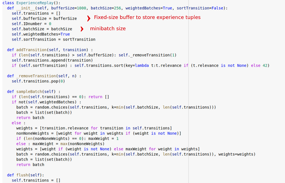
The following screen shot is the experience replay for a batch size of 3.

Learner Class
This class takes the input of Q Network, state Space & action Space, and the discount factor (gamma). Here we use the algorithm "SARSA", which is an online updating method for RL. Note that the Q learning is offline method. Moreover, the SARSA algorithm can work both on-policy and off-policy.
In the learner class we have to specify an optimizer! We can set to Adam optimizer or Stochastic gradient descent (SGD) or any other optimizer. The learn method in the Learner Class uses algorithm of either "SARSA" or "QLEARNING". Here we will compute Q(St, At) and Q(St+1, At+1). The error is estimated using square error function.
errors = torch.square(target - Q_St_At)
Training Loop
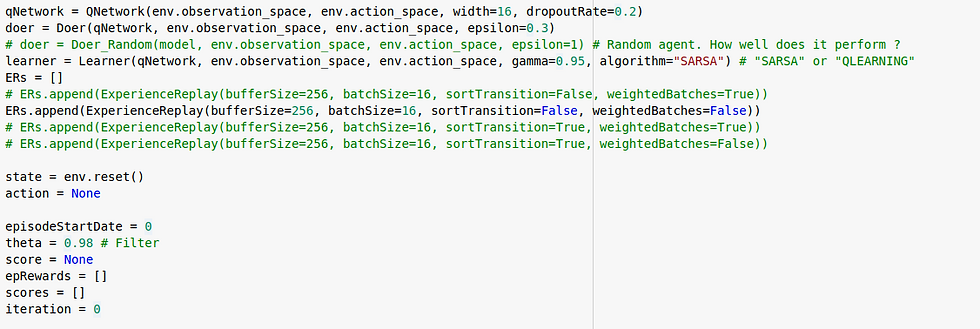
Let us initialize the training loop. Let us set the dropout of 0.2, gamma of 0.95 as follow;
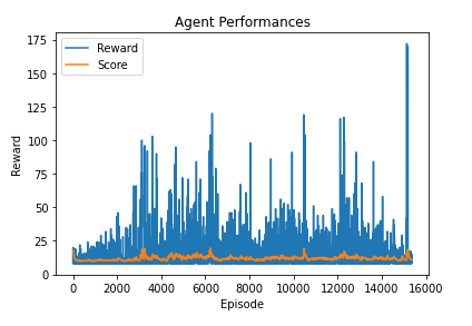
Following is the performance. We can see a very high reward at around 16000 episode.
Now let us set the dropout of 0.4 and see the performance. This appears to be good & the reward is high at around 8000 episode.

Now let us set the dropout of 0.5 and see the performance;
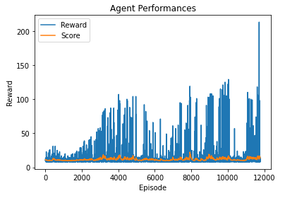
There is a slight improvement when we alter the value of dropout. From these variation 0.4 dropout seems to be better.
Let us test with the LeakyReLU(); The performance is good as well in this case.
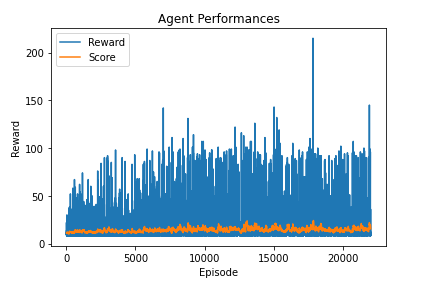
Now instead of dropout, lets play with epsilon. We didnt observe big different when we change epsilon. The following is the performance if we change the epsilon = 0.4.
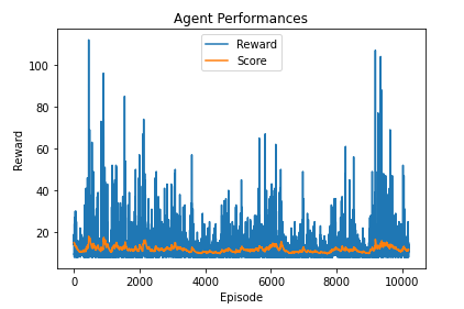
Let us check the performance of the model by varying the width.
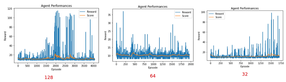
When we set the width to 32, 64 & 128, we get the following performance . It appears the low width perform better.

Let us check the performance from by varying the batch size.The following is the performance at different batch size. The small batch size it good compare to the larger one.
The following is the a short video. Unfortunately we could not train for long period. Mostly because my machine causes issues.
References:


Comments